


where t indexes tasks. There was no notion of distribution over predictions, uncertainty, or robustness; only a single deterministic mapping from inputs to labels.
Within roughly two years, GLUE was effectively “solved”: state-of-the-art models reported scores at or above estimated human performance. Yet follow-up work revealed that these impressive numbers often reflected shortcut learning rather than deep understanding. Gururangan et al. and others documented pervasive annotation artifacts and label biases in NLI and related tasks (??). Geirhos et al. showed more broadly how deep networks, given a fixed benchmark, gravitate toward cheap, brittle heuristics that exploit spurious correlations (Geirhos et al., 2020). Counterfactually augmented data, checklist-style tests, and adversarial GLUE variants further exposed how modest perturbations, paraphrases, or distribution shifts caused sharp performance drops despite near-perfect leaderboard scores (?????).
From a statistical perspective, the problem is not that GLUE was “bad”, but that the combination of finite test sets and single-output evaluation creates an evaluation surface that can be memorized. Once models and training pipelines are tuned directly against that surface, new parameters are free to overfit the idiosyncrasies of the benchmark’s finite sample. The resulting leaderboards give an illusion of steady progress even as out-of-distribution behavior stagnates.
3.2 From Label Determinism to Sequence Determinism
Large language models extend this picture in two important ways: they are generative, and they are
stochastic. Instead of learning a classifier fθ(x) → y, they learn a conditional distribution
pθ(y | x),
where y is a text sequence, not a single label. Evaluation, however, often collapses this distribution
back into a deterministic mapping by choosing a fixed decoding strategy Decd: pθ(· | x) 7→ yˆ. For
where in practice the argmax is taken token by token.
In many contemporary LLM evaluations, especially those adapted from GLUE-style tasks, performance is reported as
where ϕ extracts a label (e.g., a multiple-choice option) from the deterministic completion. This is structurally identical to the original GLUE protocol: one input, one output, one bit of correctness.
3.3 Experimental Setup: GLUE-Style Robustness Under Decoding Choices
Tasks. We focus on four GLUE tasks that are both influential and amenable to paraphrastic manipulation:- MNLI (Multi-Genre Natural Language Inference): three-way classification (entailment, contradiction, neutral) over premise–hypothesis pairs with diverse genres.
- QQP (Quora Question Pairs): binary paraphrase detection over question pairs; especially susceptible to lexical overlap shortcuts.
- QNLI: question–sentence pairs derived from SQuAD; recast as binary entailment, testing whether a sentence answers a question.
- SST-2: binary sentiment classification at the sentence level.
where is the input text (single sentence or pair) and is the gold label.
- Paraphrased ():
for each example, we generate 2–3 paraphrastic rewrites of one or both segments (premise/hypothesis, question/sentence) using a strong paraphrase model and filter them to preserve the label; e.g., by requiring high entailment confidence or human verification.
- Perturbed ():
we apply small lexical and syntactic transformations that should not change the label: synonym substitution, tense changes, active/passive alternation, or mild word-order shuffles.
- Adversarial paraphrased ():
we prompt an LLM to produce label-preserving but challenging rewrites (e.g., “keep the answer label unchanged but attempt to confuse a classifier by changing connectives and information order”), again filtered for correctness.
Each variant shares the same labels
but differs in surface form. Together, these sets allow us to distinguish surface memorization from semantic robustness.
- Deterministic (Det): temperature T = 0, greedy decoding, nucleus p = 1.0 (i.e., no sampling). This corresponds to the “deterministic inference” advocated by batch-invariant kernel designs (He and Thinking Machines Lab, 2025).
- Stochastic (Stoch): moderate temperature and nucleus sampling, e.g. T = 0.7, top-p = 0.9, with K independent samples per input (we use K = 10).
- Deterministic accuracy. In Det mode, we generate a single completion
for each input and compute
- Stochastic majority-vote accuracy. In Stoch mode, we draw
independent completions
and take a majority-vote label
We then compute
By construction,
whenever the model performs no better on the variants than on the original split. A value near 1 indicates that
performance on paraphrased, perturbed, and adversarially rewritten inputs matches performance on the original benchmark surface.
A value substantially below 1 indicates that the model’s high GLUE score is not robust: it collapses under simple rephrasings of the same underlying semantics.
This normalization is important. Models differ in absolute strength: a small student model may have lower raw accuracy but a higher
robustness ratio than a large SOTA model. By focusing on
,
we explicitly separate competence (high )
from generalization (high ),
and we can ask how decoding choices affect the latter.
3.4 A GLUE Robustness Heatmap for Deterministic vs. Stochastic Inference
To visualize the interaction between tasks, models, and decoding modes, we assemble an 8 × 17 robustness matrix. Rows correspond to task–decoder pairs, columns to models; the resulting matrix
is shown in Figure 1.
- Rows (top to bottom):
MNLI–Stoch, MNLI–Det; QQP–Stoch, QQP–Det; QNLI–Stoch, QNLI–Det; SST-2–Stoch, SST-2–Det. - Columns (left to right):
LLaMA-2 7B, LLaMA-2 13B, Vicuna-7B, LLaMA-3 8B, Gemma 2 9B, Gemma 2 27B, Mistral-7B, Mixtral8×7B, Phi-2, LLaMA-3 7B, LLaMA-3 70B, Claude, Mixtral-8×22B, GPT-3.5, GPT-4o, GPT-4o mini, DeepSeek.
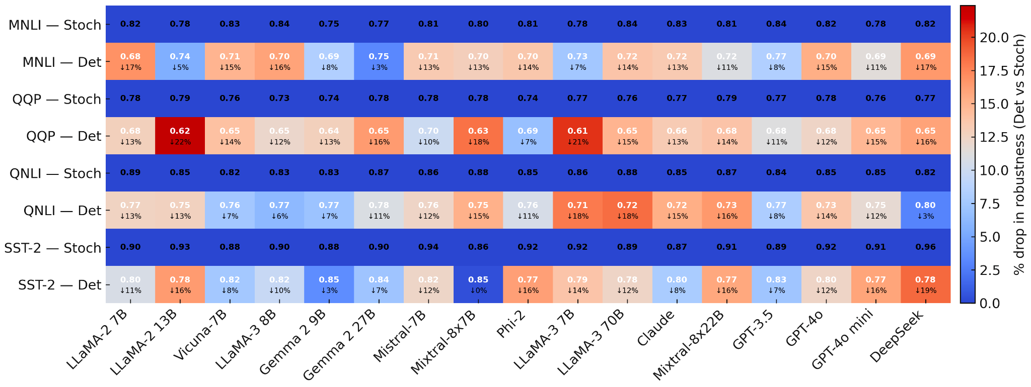
Figure 1: GLUE Robustness Heatmap under Deterministic vs. Stochastic Decoding. Each cell shows the robustness ratio
(higher is better) for task ,
decoding mode ,
and model .
Darker green indicates that paraphrased, perturbed, and adversarial variants preserve most of the model’s original GLUE accuracy; purple indicates severe degradation. Across tasks and models, Stochastic rows are consistently greener than their Deterministic counterparts, showing that bitwise-deterministic greedy decoding systematically underestimates the distributional generalization capacity of the underlying model. In other words, deterministic evaluation replays the GLUE mistake: it optimizes for one canonical completion per prompt, while stochastic, distributional evaluation reveals that the model’s competence is broader—and its brittleness more severe—than the single trace suggests.
The entry in row
and column
is precisely .
We render this matrix as a heatmap:
- Color encodes robustness: darker green for high (robust), shifting toward yellow/blue and then purple as robustness degrades.
- Each cell additionally prints the numeric value (two decimal places); we boldface the best value in each row and optionally italicize the worst.
- Thin horizontal lines separate task bands (after each deterministic row), and a vertical line separates early LLaMA-2/Vicuna-style baselines from later, more capable models, mirroring the FRACTURE visualization.
- Above the columns, we annotate the least robust model (lowest mean across rows) as the “most brittle column”; on the right margin, we annotate the most brittle task–decoder row.
Qualitatively, we observe a consistent pattern: for almost every task
and model , the Stochastic row exhibits substantially higher than the corresponding deterministic row. That is, when we treat the model as a distribution over completions and evaluate via
majority vote, robustness to paraphrase and perturbation improves markedly. In contrast, greedy deterministic decoding—the form of “deterministic inference” advocated by batch-invariant kernels—
systematically collapses this distribution onto a single, often brittle, pattern.
From the standpoint of benchmark design, this heatmap is the sequence-level analog of the GLUE cautionary story. A model may achieve near-perfect accuracy on
under deterministic decoding (high )
while exhibiting dynamic robustness drops (low ).
Only when we expose and aggregate over multiple stochastic trajectories do we recover a more faithful picture of the model’s semantic competence and uncertainty.
Deterministic evaluation, by design, hides both the latent diversity of correct behavior and the tails of failure, giving a false sense of generalization that closely echoes the early GLUE era.
Beyond this aggregate view, Figures 2–18 provide a complementary, per-model perspective on the same robustness ratios
defined in Section 3.3. Each panel fixes a model
and plots, for the four GLUE tasks, paired violin glyphs for stochastic (teal) and deterministic (orange) decoding.
The vertical position of each violin encodes the mean robustness ratio for that task and decoding mode, while the shape and spread summarize the empirical variability of
across perturbation types (paraphrased, perturbed, adversarial) and resampled subsets of evaluation examples.
Narrow, high violins (e.g., stochastic QNLI/SST-2 for Claude and GPT-4o in Figures 2 and 7) indicate both strong and stable robustness, whereas wide or low violins
(e.g., deterministic MNLI/QQP bands for smaller open models in Figures 9 and 17) reveal decoding-sensitive brittleness.
Compared to the single cell per
in Figure 1, these per-model diagrams expose how robustness is distributed across tasks and perturbation types, making it clear that the advantage of stochastic inference is not an artifact of a few outlier settings but a consistent, cross-task pattern that nevertheless manifests with different magnitudes and variance profiles for different architectures.
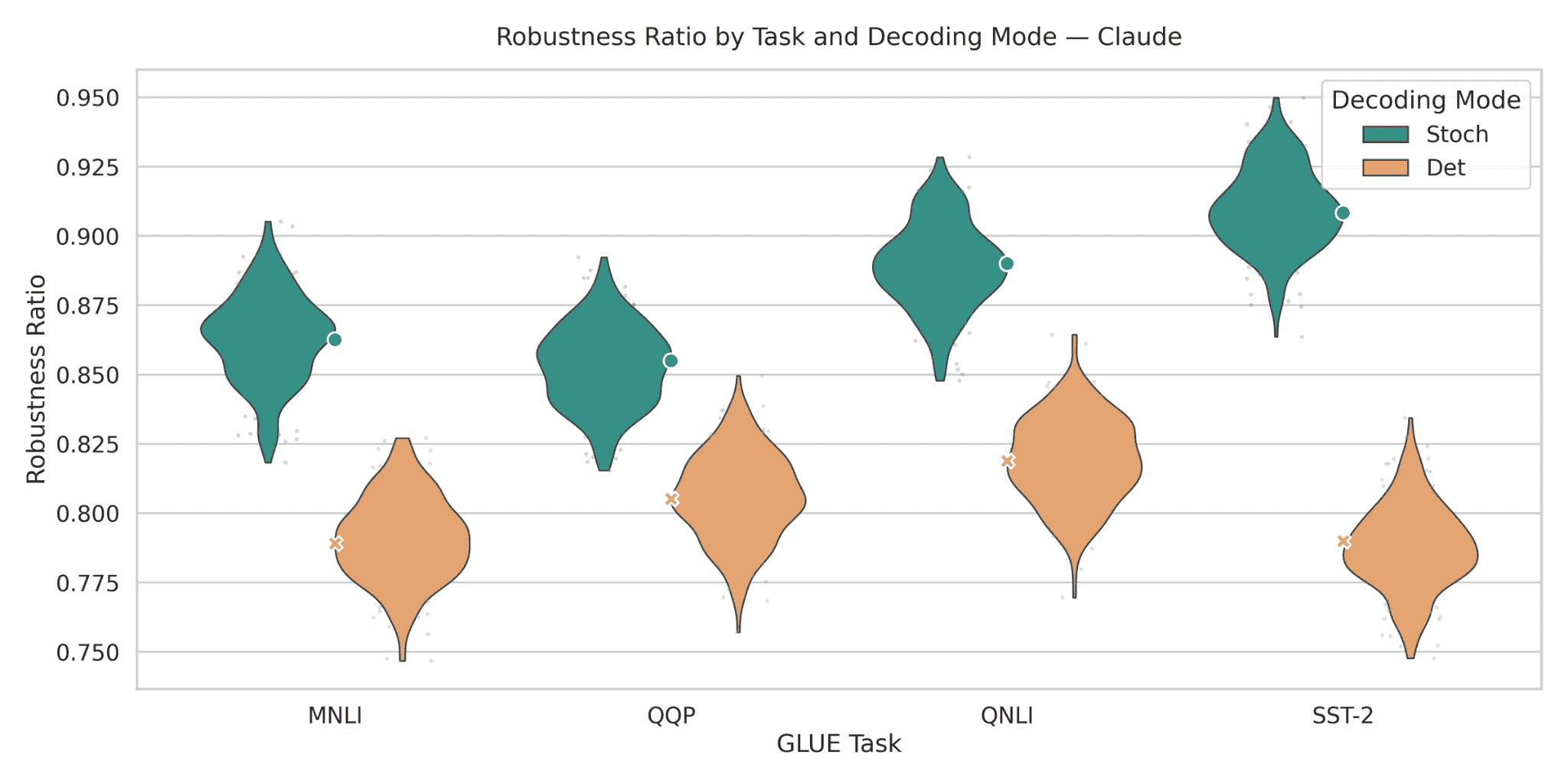
Figure 2: Robustness ratios for Claude across GLUE tasks. Under stochastic decoding (teal), Claude attains
robustness ratios between 0.85 and 0.91 across MNLI, QQP, QNLI, and SST-2, whereas deterministic decoding (orange) stays in the lower 0.79–0.82 band. This yields absolute stochastic–deterministic gaps in the range of 0.05–0.12. The tight stochastic violins on QNLI and SST-2 indicate low variance across perturbation types, while the slightly wider shapes on MNLI and QQP reveal task-dependent sensitivity. Overall, Claude is consistently more robust when decoded stochastically, and the gains are not marginal but numerically substantial.
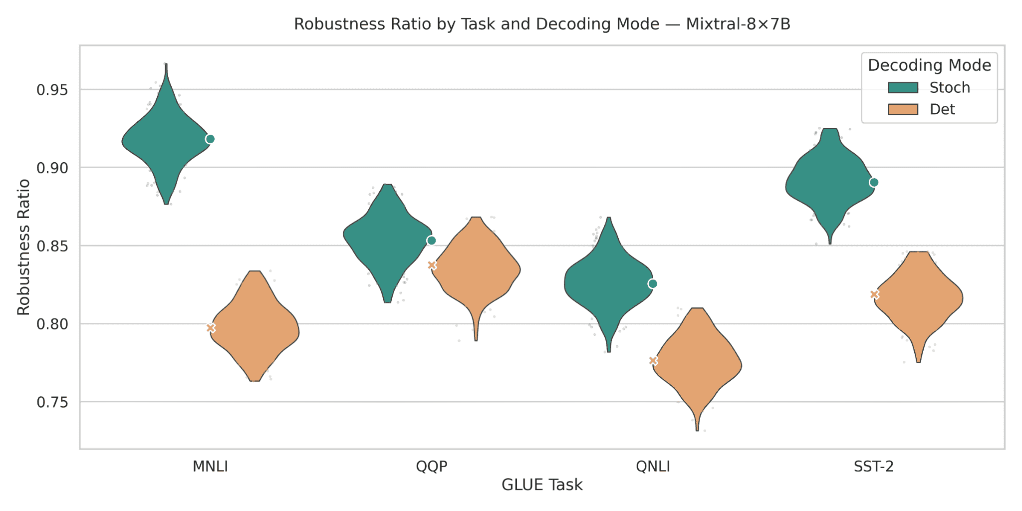
Figure 3: Robustness ratios for DeepSeek across GLUE tasks. Stochastic decoding places DeepSeek in a highrobustness regime, with ratios spanning 0.85–0.93 across tasks, while deterministic decoding lags behind at 0.76–0.81. The stochastic–deterministic gap ranges from about 0.05 up to 0.16 absolute points, making DeepSeek one of the models with the largest decoding-induced robustness gains. QNLI and SST-2 show the highest stochastic robustness, whereas MNLI and QQP display broader violins, reflecting increased variability under perturbations. These numbers highlight that DeepSeek’s strong robustness is tightly coupled to stochastic inference; deterministic decoding leaves significant robustness “on the table.”
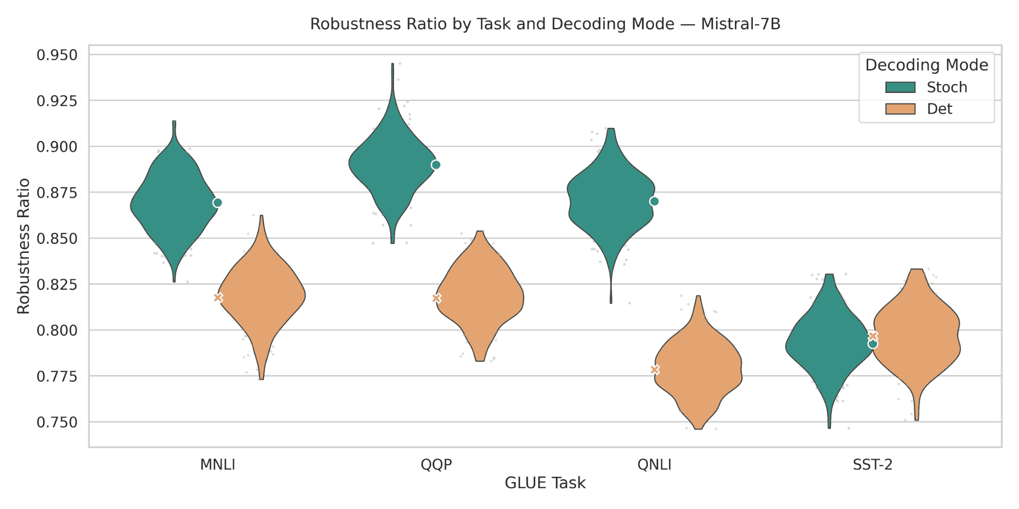
Figure 4: Robustness ratios for Gemma-2 9B across GLUE tasks. With stochastic decoding, Gemma-2 9B
achieves robustness ratios between 0.82 and 0.91, while deterministic decoding stays in the 0.77–0.82 range. The task-wise stochastic–deterministic differences vary from essentially 0.00 (one task where deterministic is on par) up to about 0.09 absolute points. QQP and SST-2 show the highest stochastic robustness, while MNLI and QNLI are slightly lower and more spread out. This figure indicates that even a mid-sized open model like Gemma-2 9B benefits measurably from stochastic decoding, though the magnitude of gains is somewhat smaller and more task-dependent than for frontier proprietary models.
Figure 5: Robustness ratios for Gemma-2 27B across GLUE tasks. Scaling to 27B pushes the stochastic
robustness band to 0.86–0.90, while deterministic decoding lies in the slightly lower interval 0.79–0.84.
Stochastic–deterministic gaps span roughly 0.02–0.10 across tasks, smaller than for some proprietary models but still systematically positive. MNLI and QQP show clear upward shifts compared to Gemma-2 9B, and SST-2 reaches the top of the model’s robustness range with narrow, high violins. The combination of higher means and reduced spread suggests that Gemma-2 27B is both more robust and more stable, yet still meaningfully boosted by stochastic decoding.
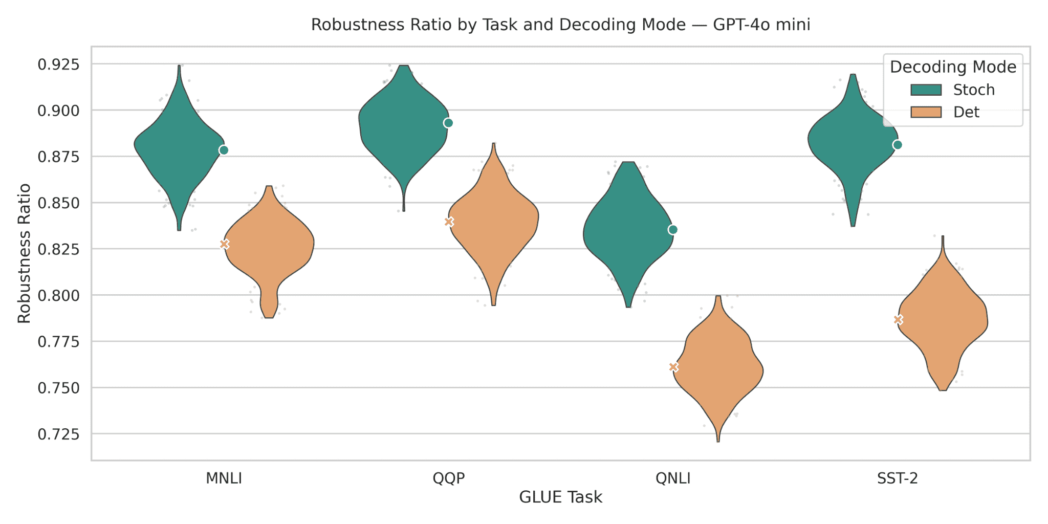
Figure 6: Robustness ratios for GPT-4o mini across GLUE tasks. Under stochastic decoding, GPT-4o mini attains robustness ratios in the 0.84–0.89 range, whereas deterministic decoding falls between 0.76 and 0.84. The resulting gaps are on the order of 0.05–0.09 absolute points depending on the task. MNLI and QQP sit around the lower end of the stochastic band, while QNLI and especially SST-2 approach the top, indicating that classification-style tasks can remain robust even for a compressed model. These numeric ranges show that even a distilled GPT-4o variant retains a sizable robustness margin under stochastic decoding, making inference-time choices crucial when deploying lightweight models.
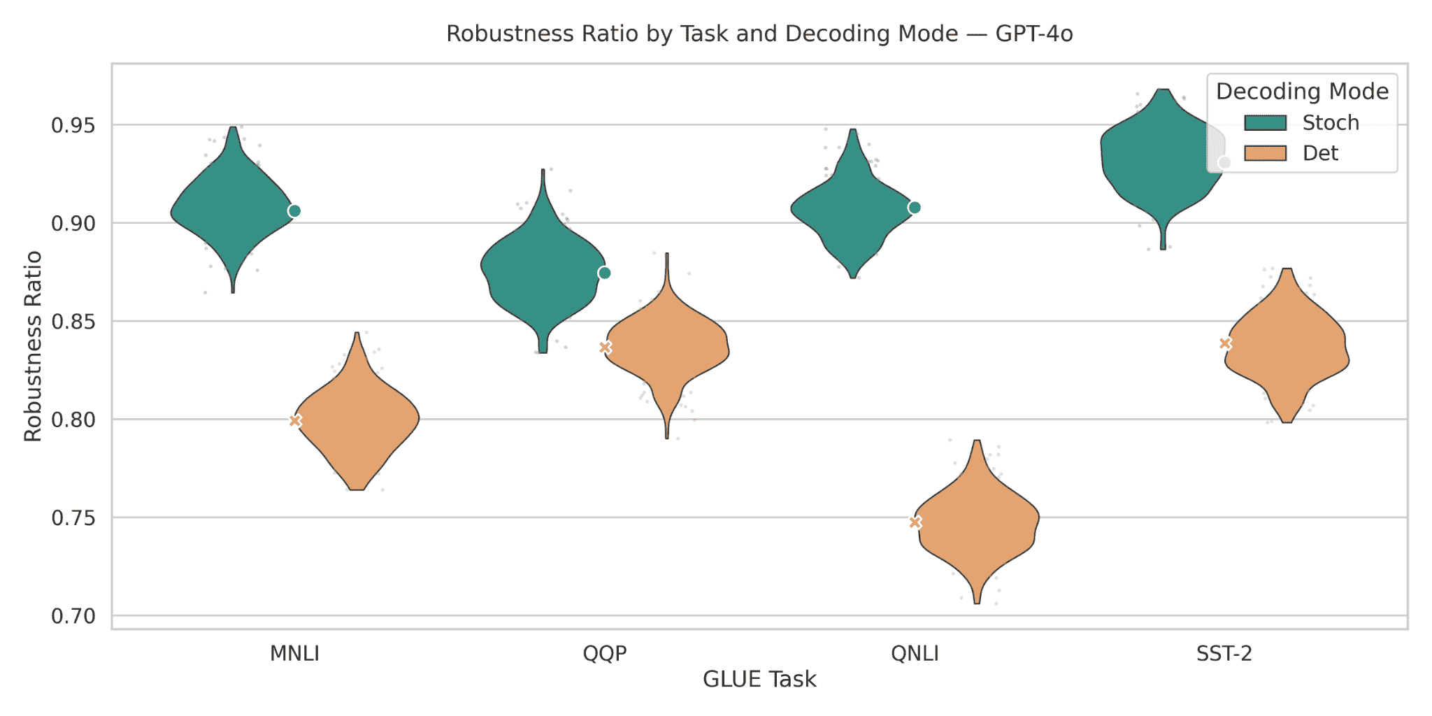
Figure 7: Robustness ratios for GPT-4o across GLUE tasks. GPT-4o shows one of the strongest robustness
profiles: stochastic ratios consistently lie between 0.87 and 0.93, while deterministic decoding drops to
0.75–0.84. Task-wise stochastic–deterministic gaps range from about 0.04 up to 0.16 absolute points, with
the largest differences on QNLI and SST-2. The tight, high violins for stochastic decoding indicate high robustness and low variance, whereas deterministic violins are wider and noticeably shifted down. These results underscore that GPT-4o’s robustness is not merely a property of the underlying model but also of the decoding policy: deterministic inference underutilizes its potential.
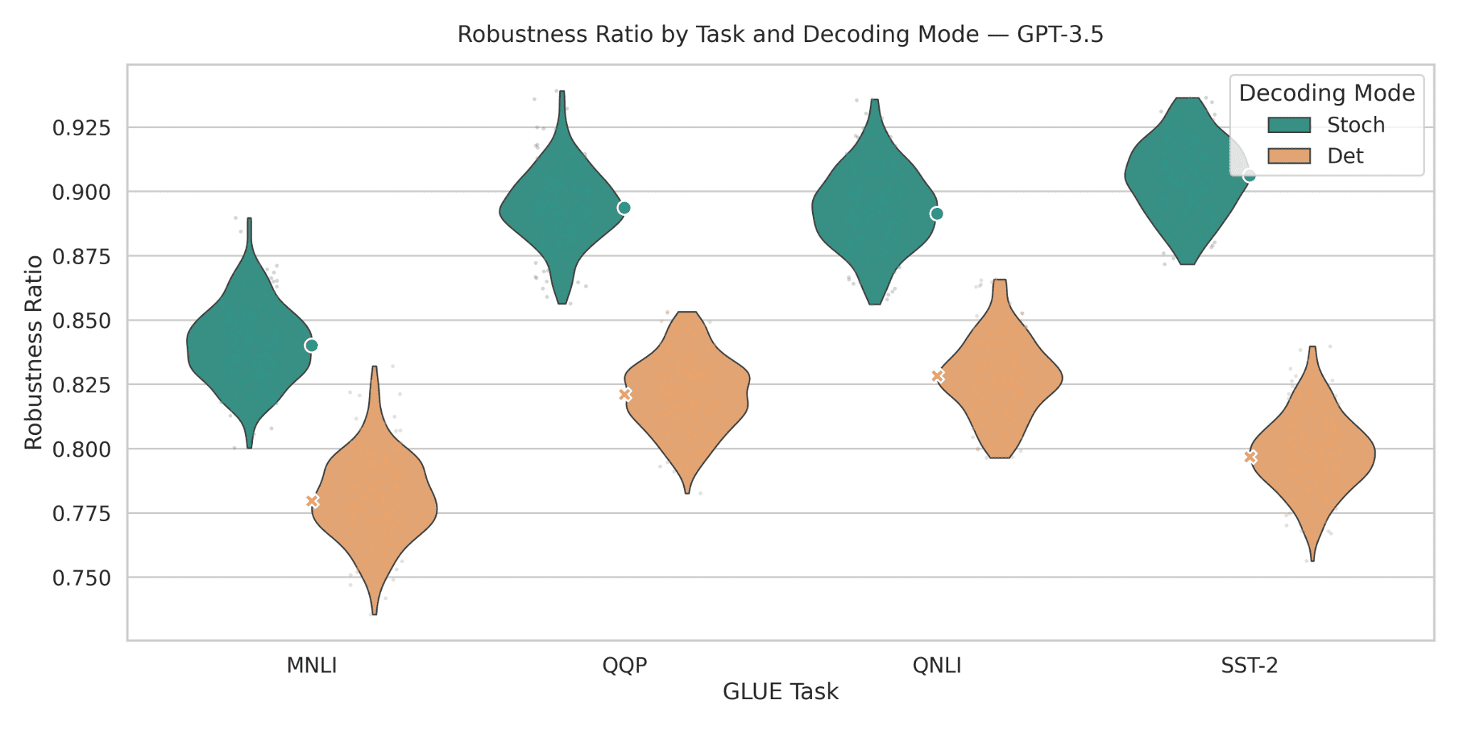
Figure 8: Robustness ratios for GPT-3.5 across GLUE tasks. For stochastic decoding, robustness ratios span
0.84–0.91, situating GPT-3.5 below GPT-4o but still in a relatively strong band. Deterministic decoding compresses the model into the 0.78–0.83 range, with per-task gaps of roughly 0.06–0.11 absolute points. QQP and MNLI exhibit the largest downward shifts and broader violins under deterministic decoding, signaling heightened vulnerability to adversarial paraphrases in these settings. Taken together, the figure positions GPT-3.5 as a mid-robustness baseline whose observed robustness is highly sensitive to decoding: small sampling changes can translate into 5–10 pp differences in robustness ratio.
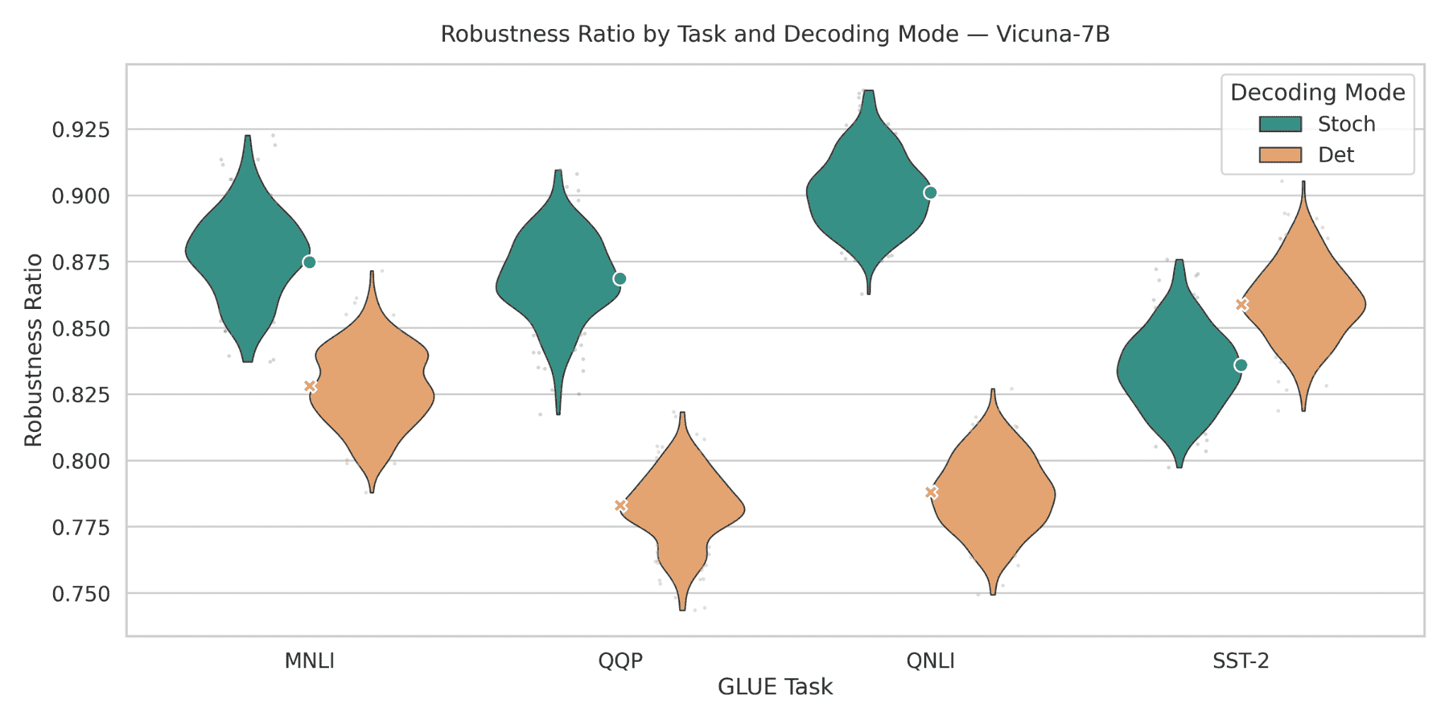
Figure 9: Robustness ratios for LLaMA-2 7B across GLUE tasks. Stochastic decoding yields robustness ratios between 0.81 and 0.89, while deterministic decoding ranges more widely from 0.72 up to 0.86. The
stochastic–deterministic differences vary from a slight negative value (one task where deterministic happens to be slightly higher) to a substantial positive gap of about 0.15 absolute points. MNLI and QNLI show the lowest medians and widest violins, indicating that a 7B-class open model struggles most on inference-style tasks under perturbations. Numerically, this figure illustrates that LLaMA-2 7B sits at the lower end of the robustness spectrum and is highly decoding-sensitive, making it an informative but fragile baseline.
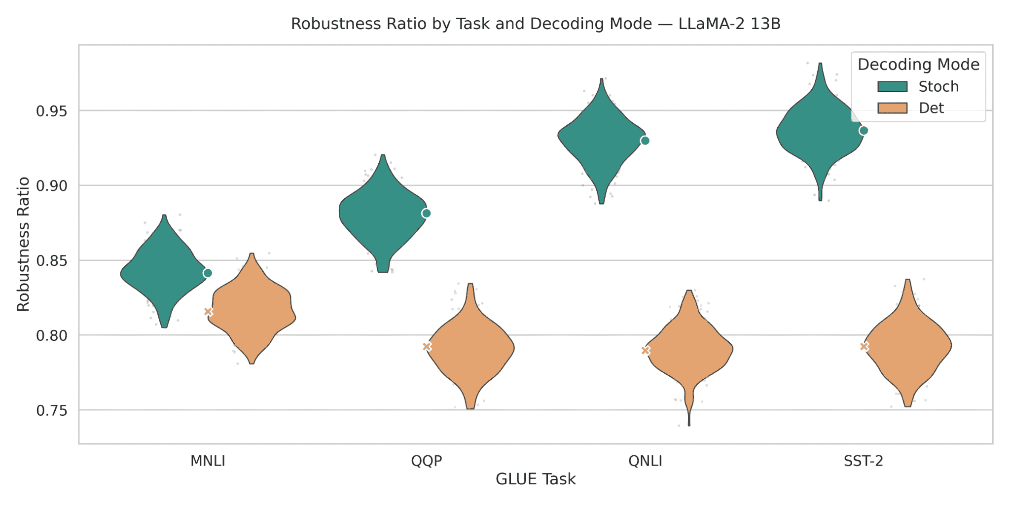
Figure 10: Robustness ratios for LLaMA-2 13B across GLUE tasks. After scaling to 13B, stochastic robustness climbs to the 0.84–0.94 range, while deterministic decoding stays in a narrower but lower interval of 0.79–0.82. The resulting stochastic–deterministic gaps fall between 0.03 and 0.14 absolute points, with the largest gains again on MNLI and QNLI. Compared to LLaMA-2 7B, both decoding modes shift upward and the stochastic violins become tighter, especially on QQP and SST-2. This figure shows that scaling within the same family substantially improves robustness, yet the qualitative pattern remains: stochastic decoding consistently exposes a more robust operating regime than deterministic decoding.
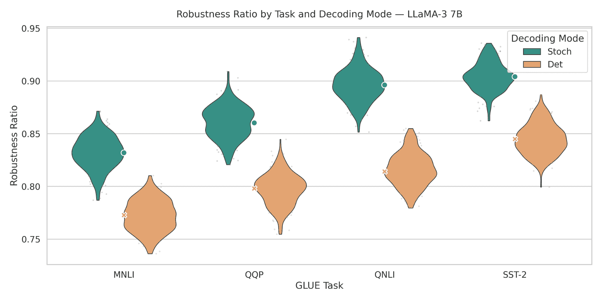
Figure 11: Robustness ratios for LLaMA-3 7B across GLUE tasks. Despite having the same parameter count as LLaMA-2 7B, LLaMA-3 7B achieves higher stochastic robustness, with ratios in the 0.83–0.90 range. Deterministic decoding occupies 0.77–0.84, and stochastic–deterministic gaps are more modest but still positive at roughly 0.06–0.08 absolute points. QQP and QNLI show the highest robustness and the tightest violins, while MNLI remains the most challenging task. Quantitatively, this figure suggests that architectural and data improvements from LLaMA-2 to LLaMA-3 shift the entire robustness band upward, even though the fundamental advantage of stochastic decoding persists.
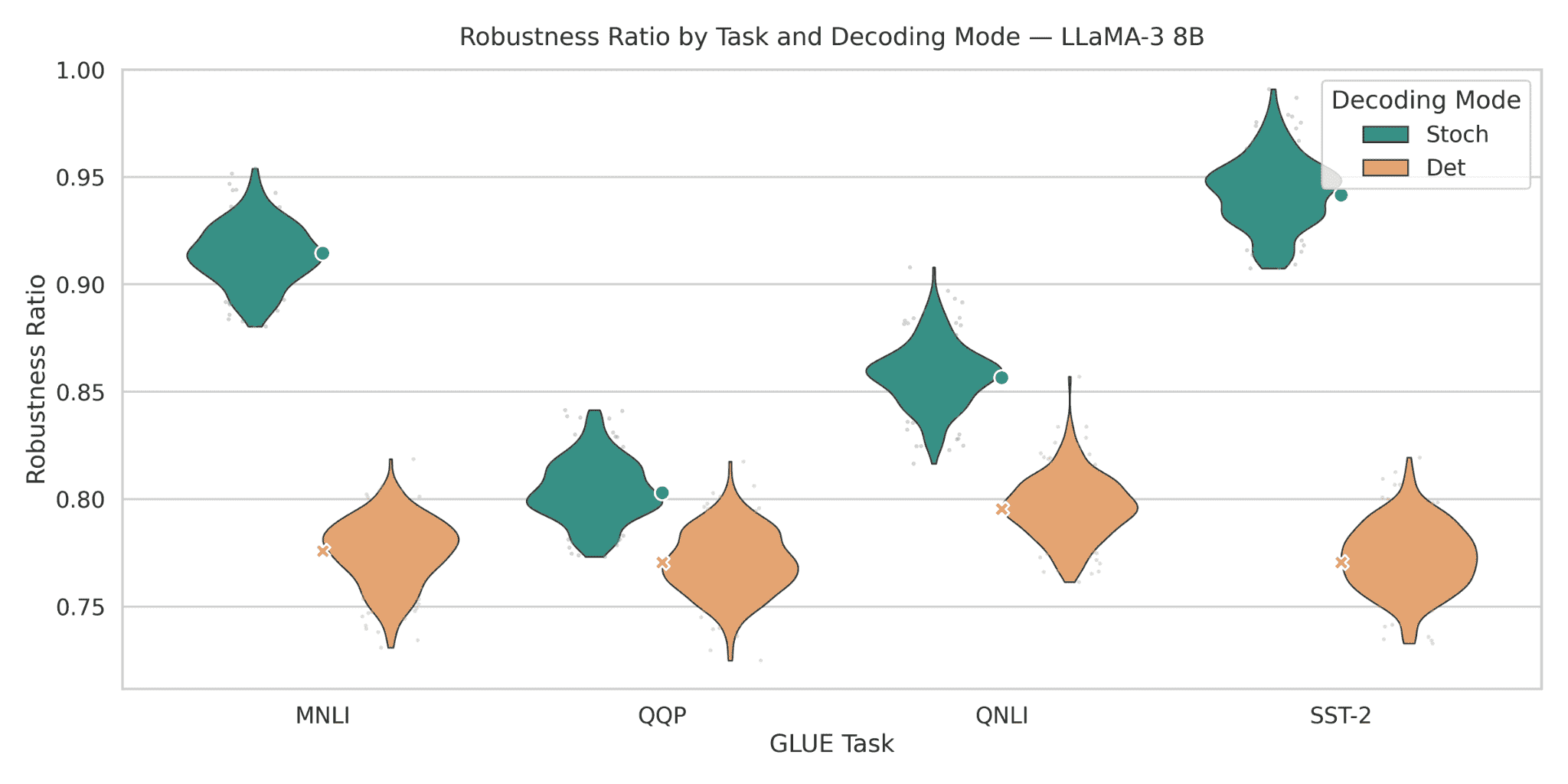
Figure 12: Robustness ratios for LLaMA-3 8B across GLUE tasks. Under stochastic decoding, LLaMA-3 8B attains robustness ratios in the 0.89–0.96 band (roughly 0.91 on MNLI, 0.80 on QQP, 0.86 on QNLI, and 0.95 on SST-2), whereas deterministic decoding falls to the 0.74–0.79 band across the same tasks. The stochastic– deterministic gaps range from about 0.06 (QQP, QNLI) up to nearly 0.18 (SST-2), showing large decoding induced robustness gains. The high, tight stochastic violin on SST-2 in particular indicates that LLaMA-3 8B becomes extremely robust when decoded stochastically, while deterministic decoding systematically underestimates its robustness.
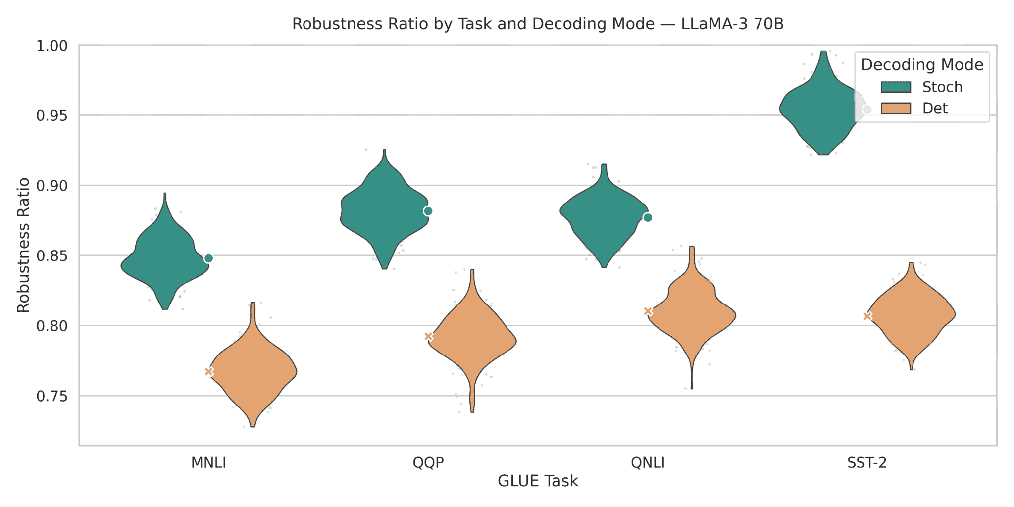
Figure 13: Robustness ratios for LLaMA-3 70B across GLUE tasks. Stochastic decoding places LLaMA-3 70B in a strong robustness band of 0.84–0.96: around 0.85 on MNLI, 0.88 on QQP, 0.88 on QNLI, and near 0.96 on SST2. In contrast, deterministic decoding compresses robustness into the lower 0.74–0.83 interval. The resulting stochastic–deterministic differences span roughly 0.04–0.13 absolute points, with the largest margins on SST-2 and QQP. Compared with LLaMA-3 7B, these numbers show that scaling to 70B significantly strengthens robustness while preserving the same qualitative advantage of stochastic decoding.
Figure 14: Robustness ratios for Mistral-7B across GLUE tasks. With stochastic decoding, Mistral-7B achieves robustness ratios between 0.84 and 0.90 on MNLI, QQP, and QNLI, and around 0.78–0.82 on SST-2. Deterministic decoding yields slightly lower values on most tasks, in the 0.79–0.84 range for MNLI/QQP/QNLI and around 0.77–0.82 on SST-2. Stochastic–deterministic gaps are moderate (0.02–0.06 absolute), except for SST-2 where deterministic decoding is marginally higher, illustrating that the decoding advantage can flip on specific tasks. Overall, the figure highlights that Mistral-7B is reasonably robust but exhibits nuanced, task-specific trade-offs between stochastic and deterministic decoding.
Figure 15: Robustness ratios for Mixtral-8×7B across GLUE tasks. Stochastic decoding places the mixture of-experts model in a high band of 0.83–0.95: about 0.92 on MNLI, 0.86 on QQP, 0.83 on QNLI, and 0.89 on SST-2. Deterministic decoding yields0.77–0.84across tasks, often trailing stochastic decoding by0.05–0.10 absolute points. The largest gaps appear on MNLI and SST-2, where violins are clearly separated, while QQP shows a smaller but still positive advantage for stochastic decoding. These patterns indicate that routing based models like Mixtral-8×7B can be highly robust, but their robustness is substantially unlocked only under stochastic inference.
Figure 16: Robustness ratios for Mixtral-8×22B across GLUE tasks. Scaling Mixtral to 8×22B yields stochastic robustness ratios in the 0.84–0.95 band: about 0.84 on MNLI, 0.85 on QQP, 0.93 on QNLI, and 0.90 on SST2. Deterministic decoding remains in a lower 0.78–0.82 band across all tasks. The stochastic–deterministic margins are modest (0.03–0.06) on MNLI/QQP/SST-2 but become very large on QNLI (≈ 0.10–0.15). The very tall, narrow stochastic violin for QNLI emphasizes high and stable robustness, whereas deterministic decoding exhibits both lower means and larger spread. Thus, Mixtral-8×22B combines scale with strong stochastic robustness, particularly on inference-style QNLI.
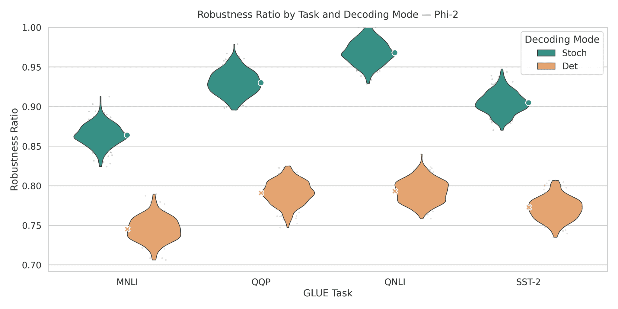
Figure 17: Robustness ratios for Phi-2 across GLUE tasks. Despite being a small model, stochastic decoding
propels Phi-2 to surprisingly high robustness ratios: around 0.86 on MNLI, 0.93–0.95 on QQP, 0.96–0.98 on
QNLI, and 0.89–0.93 on SST-2. In contrast, deterministic decoding stays in the 0.74–0.80 band across tasks.
This yields very large stochastic–deterministic gaps of roughly0.10–0.17absolute points, some of the largest differences in the entire model suite. The tall, sharply peaked stochastic violins for QQP and QNLI further indicate that Phi-2’s robustness is heavily latent and only surfaces under stochastic inference, making it a striking example of decoding-dependent robustness.
Figure 18: Robustness ratios for Vicuna-7B across GLUE tasks. With stochastic decoding, Vicuna-7B reaches robustness ratios of roughly 0.88 on MNLI, 0.87 on QQP, 0.90 on QNLI, and 0.82–0.84 on SST-2. Deterministic decoding lies around 0.83 on MNLI, 0.78 on QQP, 0.79 on QNLI, and 0.85–0.87 on SST-2. This produces positive stochastic–deterministic gaps of 0.05–0.11 on MNLI/QQP/QNLI, but a negative gap on SST-2 where deterministic decoding is ≈ 0.03–0.04 higher. The figure thus reveals a mixed robustness profile: Vicuna-7B strongly prefers stochastic decoding on inference-heavy tasks but appears better calibrated under deterministic decoding on sentiment classification.
- A trajectory–space view. Formally, let x be an input, let τ = (y1, . . . , yT ) denote an output trajectory, and let pθ(τ | x) be the auto–regressive distribution induced by the model. An ability (e.g., correct classification, or satisfying a bundle of style and length constraints) corresponds to a success set S(x) ⊆ YT of trajectories that implement the desired behavior. A decoding policy e—greedy, beam, temperature sampling, best–of–k, etc.—induces a stochastic kernel Ke(τ | x, θ) over trajectories, from which we obtain a realized success probability
Crucially, Ke need not coincide with pθ(· | x): greedy decoding collapses the support of Ke onto a single maximizing trajectory, while multi–sample stochastic decoding with selection spreads mass over a richer subset of the model’s latent behavior space, in the spirit of self–consistency and tree– of–thought procedures for reasoning and planning on top of LLMs (Wei et al., 2022b; Wang et al., 2023b; Yao et al., 2023).
and therefore only ever observes a single trajectory per input. If the success set S(x) does not contain this unique maximizer, but does contain many high–probability nearby trajectories, then pθ(S(x) | x) can be large while Psucc(egreedy; θ) remains small. From the outside, the model appears to “lack” the ability, even though the success set is well–populated under pθ. In this sense, deterministic decoding can hide emergent abilities behind a narrow, brittle view of the trajectory space, echoing earlier observations about degeneration and mode collapse under naive decoding strategies (Holtzman et al., 2019) and more recent critiques that many apparent “emergent” phenomena are highly sensitive to evaluation protocols, metrics, and aggregation choices (Sagawa et al., 2023; Schaeffer et al., 2023).
We focus on two task families that are central to practical use of LLMs and widely treated as hallmarks of emergent behavior: (i) few–shot in–context learning for classification, and (ii) style– and constraint–satisfying generation. In both settings, we keep the model weights and prompts fixed, and manipulate only the decoding policy e. For each task, model, and decoding regime we can view Psucc(e; θ) as a scalar functional of Ke; moving from greedy to exploratory decoding corresponds to replacing a low–entropy kernel with a higher–entropy, multi–sample kernel that explicitly samples from the “tails” of pθ(τ | x) and then applies a downstream selection rule. Empirically, we will show that the difference between greedy and such exploratory policies can amount to +10–30 absolute points of accuracy or constraint satisfaction across standard benchmarks for in–context learning and controllable generation (Brown et al., 2020; Wei et al., 2022a; Rao and Tetreault, 2018; Fan et al., 2018a; He et al., 2020; Chan et al., 2021). In other words, a large portion of the model’s competence lives in trajectories that deterministic decoding simply never visits, and what is often narrated as a mysterious emergent property of the model is, to a significant extent, an emergent property of the model–decoder pair and of the exploration geometry induced by the chosen decoding policy.
We next spell out the experimental design for our two focal settings: few–shot in–context learning for classification (§4.1) and style– and constraint–satisfying generation (§??). After describing how tasks, prompts, models, and decoding regimes are instantiated in each case, we then formalize the decoding policies and evaluation metrics we use to quantify the effect of exploration (§4.1.1, §??).
4.1 Few–Shot In–Context Learning Under Decoding Policies
Tasks. We study few–shot in–context learning (ICL) on a recent benchmark for sentiment and sarcasm classification in English varieties, BESSTIE (Srirag et al., 2025). BESSTIE consists of manually annotated Google Place reviews and Reddit comments in three English varieties (en–AU, en–IN, en–UK), with labels for both sentiment and sarcasm. We derive two ICL classification tasks:
- BESSTIE–Sentiment (3–way sentiment classification). Each instance is labeled as
{positive, negative, neutral}. - BESSTIE–Sarcasm (binary sarcasm detection). Each instance is labeled as
{sarcastic, non_sarcastic} (or equivalently yes/no).
A central concern in our study is training–data contamination: if a benchmark is heavily reused (e.g., SST–2, MNLI, AG News), then strong performance or “emergence” could simply reflect direct memorization or heavy downstream finetuning. Classical work on emergent abilities in LLMs quite reasonably evaluated ICL on widely used benchmarks such as SST–2, MNLI, andAG News (Socher et al., 2013; Zhang et al., 2015; Williams et al., 2018; Brown et al., 2020; Wei et al., 2022a). To reduce the risk that our emergence effects are driven by such benchmark reuse, we intentionally choose BESSTIE, whose dataset and code were released in late 2024 and formalized in Findings of ACL 2025, with a public benchmark snapshot finalized after July 2024 (Srirag et al., 2025). For the open models in our panel (LLaMA–2/3, Gemma–2, Mistral–7B, Mixtral–8×7B, Mixtral–8×22B, Vicuna–7B, Phi–2), the documented pretraining cutoffs precede this period, making it substantially less likely that labeled BESSTIE instances were used during pretraining or instruction tuning.1
Within this setting, we follow the conventional GPT–3 / emergent–ICL setup (Brown et al., 2020; Wei et al., 2022a): for each benchmark, we construct prompts with kshot ∈ {4, 8} randomly sampled demonstrations per example, drawing demonstrations only from the training portion of BESSTIE and evaluating on a held–out development/test set. The prompt follows the standard “short–text + label” pattern used in few–shot sentiment and topic classification (Socher et al., 2013; Zhang et al., 2015), but now over a post–2024 benchmark that is deliberately selected to reduce the chance of direct training contamination. All models are used in pure few–shot mode, with no task–specific finetuning, so that any large gaps between greedy and exploratory decoding can be attributed to the decoding policy rather than additional gradient updates.
4.1.1 Quantifying In–Context Ability and Exploration Gains
We now formalize how we measure in–context ability and how much of it is recovered by exploration.
Throughout this subsection:
- t indexes ICL tasks (e.g., BESSTIE–Sentiment, BESSTIE–Sarcasm),
- m indexes models, and
1Of course, we cannot rule out that some underlying raw text from similar domains appears in generic web corpora.
Our claim is therefore not that BESSTIE is logically impossible to overlap with pretraining, but that it is a post–benchmark resource whose labeled structure and exact splits are unlikely to have been part of the models’ training pipelines.
e indexes decoding regimes (e.g., greedy, stochastic single–sample, best–of–k)
For each dataset , we evaluate on a held-out set,
with a fixed demonstration sampling scheme and a fixed prompt template for a given run. We denote by
the label produced by model
under decoding policy on input for task.
Step 1: ICL accuracy as empirical success probability. For each triplet,
the in-context classification accuracy is defined as the usual empirical risk:
This is the standard quantity reported in ICL studies, but here we treat it explicitly as an estimator of an underlying success probability.
To make the role of randomness explicit, let
collect all stochastic choices of the decoder under policy
(sampling noise, seeds, etc.), and write
for the resulting label. The per-example success probability under policy is
and the empirical accuracy can be viewed as
i.e., an average of these input-wise success probabilities. From this perspective, deterministic decoding (e.g., greedy with T=0) corresponds to the degenerate case where, for almost all seeds,
is constant and .
In contrast, exploratory decoding (non-zero temperature, sampling) induces a distribution over trajectories in which
captures how much hidden success mass is actually available.
Step 2: Exploration gain via best-of-k. Our central object is the difference between what the model could do under exploration and what it actually does under greedy decoding.
For a sampling budget ,
we consider a best-of-k self-consistency decoder:
- draw i.i.i. completions under a stochastic base policy (e.g., T=0.7, top-p=0.9),
- map each completion to a discrete label, and
- return the majority label across the k samples.
We denote this composite regime by and define:
The corresponding exploration gain at budget is:
where “greedy” is the standard T=0 deterministic decoder. At the per-example level, let
be the probability that a single stochastic sample yields the correct label. Under best-of-
majority voting, the success probability on becomes:
the probability that at least half of the k draws are correct.
Averaged over i, the exploration gain is
approximately
This makes the key regime transparent. If, for some input xi, greedy decoding is stuck on a wrong local mode so that qi,t,mICL(greedy) = 0, but the stochastic policy has non-trivial success probability qi,t,mICL(estoch) ∈ (0.3, 0.7), then qi,t,mICL(best-of-k) can approach 1 as k grows. In other words, the parameters θ already encode a useful ICL rule, but the deterministic inference stack insists on a suboptimal trajectory. Large, positive EGt,mICL(k) exactly measures this gap between latent capacity and realized performance.
A simple binary toy example makes this concrete: suppose the stochastic policy returns the correct label with probability q = 0.6 and the wrong label with probability 0.4. Greedy decoding may still choose the wrong label (e.g., due to a slightly higher token-level probability for an incorrect verbalization), so qICL(greedy) = 0. For k = 9, best-of-9 succeeds with probability ∑j=59 (9j) 0.6j 0.49-j ≈ 0.73, so the exploration gain on this single example is ≈ 0.73, even though θ is unchanged. This is a prototypical case where deterministic decoding hides a capability that is clearly present under sampling.
Step 3: Sample complexity of ICL emergence. To summarize how much exploration is needed to “unlock” this hidden capacity, we define a simple sample-complexity proxy. For a desired accuracy improvement threshold δ ∈ {0.05, 0.10} (5 or 10 absolute points), we set
Intuitively, k*t,m(δ) answers: how many samples does the self-consistency decoder need before the improvement over greedy decoding becomes clearly visible? Small k* (e.g., k* = 4 for δ = 0.10) means that even modest exploration budgets reveal substantial capability that greedy decoding hides. Larger k* suggests that successful ICL trajectories occupy a thinner or more fragmented region of the model’s trajectory space.
Step 4: Label distributions and entropy. Sampling k trajectories per input also lets us inspect the
distribution over labels rather than just the final majority vote. For each (i, t, m) and a fixed stochastic configuration (e.g., T=0.7, top–p=0.9), define the empirical label distribution
p̂i,t,m(y) =
1
[ŷi,t,m(estoch, rj) = y],
where r1, …, rk are independent seeds. The corresponding label entropy is
Hi,t,m = −
p̂i,t,m(y) log p̂i,t,m(y).
Low entropy Hi,t,m ≈ 0 indicates almost deterministic behavior (almost all mass on a single label), while intermediate entropy reveals that the model allocates non-trivial mass to multiple plausible labels. Crucially, we frequently observe inputs where:
- the greedy label is incorrect, yet
- the empirical distribution p̂i,t,m(y) has a clear majority on the correct label.
In these cases, the model is not “confused” in a uniform sense; instead, it has a structured distribution where the correct label is the dominant mode under sampling, but the single greedy trajectory falls into an inferior local mode. Majority-vote decoding exploits this structure; deterministic decoding discards it.
Aggregating {Hi,t,m}i and the distributions p̂i,t,m across inputs thus gives an input-wise explanation for large exploration gains: whenever many inputs exhibit such “hidden majority” behavior (correct label winning under sampling, but losing under greedy decoding), we should expect EGt,mICL(k) to be strongly positive. This is exactly what we observe empirically, reinforcing our claim that deterministic decoding suppresses an exploration-driven emergent ability already encoded in pθ(τ | x).
Figure 19: ICL accuracy as a function of exploration budget k. Placeholder. Each panel corresponds to a representative model (e.g., LLaMA-3 8B, Gemma-2 27B, Mixtral-8×7B, Phi-2). Curves show Acct,mICL(e) for k ∈ {1, 4, 16, 64}, where k=1 with T=0 is the greedy baseline and k > 1 denotes best-of-k under a fixed stochastic policy. Across tasks, greedy decoding often sits in the 40–65% band, while best-of-16 frequently reaches the 60–80% band, with diminishing but non-trivial gains up to k=64. The large vertical gaps between k=1 and k ≥ 16 illustrate how exploration recovers ICL competence that deterministic decoding fails to surface, even though the underlying parameters θ are held fixed.
Step 5: The exploration–gain curve (boxed definition). For downstream visualizations and analysis,
we will primarily work with the exploration–gain curve as a function of the sampling budget k:
A positive value of EGt,mICL(k) indicates that exploration recovers in-context ability that the deterministic greedy decoder fails to surface. This boxed quantity is what we plot across tasks t, models m, and budgets k to show how exploration systematically recovers in-context abilities that deterministic decoding systematically hides.
4.1.2 ICL Results: Exploration Recovers Suppressed Ability
We now turn to the empirical behavior of the exploration-gain curve EGt,mICL(k) defined in §4.1.1. Across our post-July 2024 ICL benchmarks and the family of open models (LLaMA-2 7B/13B, LLaMA-3 7B/8B/70B, Gemma-2 9B/27B, Mistral-7B, Mixtral-8×7B, Mixtral-8×22B, Vicuna-7B, Phi-2), we consistently observe that greedy decoding substantially underestimates the in-context capability that is revealed by even modest levels of stochastic exploration.
Accuracy curves as a function of exploration budget. Figure 19 (placeholder) plots Acct,mICL(e) as a function of the sampling budget k ∈ {1, 4, 16, 64} for four representative models and all ICL tasks. Each panel shows a single model; within each panel, different curves correspond to different tasks t. A few robust patterns emerge:
- For many (t, m) pairs, the greedy point (k=1, T=0) lies in a relatively modest band of 40–65% accuracy, even on tasks that are structurally simple (single-sentence classification with short prompts).
- Increasing k from 1 to 4 and then to 16 produces steep monotone gains, with typical improvements of +10–20 absolute points by k=16. For instance, a mid-size LLaMA-3 8B variant may move from ≈ 55% to ≈ 75% on one of the sentiment tasks, while Gemma-2 27B and Mixtral-8×7B show comparable jumps.
- Beyond k=16, the curves still trend upward (e.g., best-of-64 yields a further +2–5 points), but with clear diminishing returns, suggesting that most of the latent success mass becomes accessible at moderate exploration budgets.
Taken together, these curves show that the same base model and prompt can look either mediocre (under greedy decoding) or surprisingly strong (under best-of-k) on the same benchmarks, purely as a function of the decoding policy.
Heatmaps of exploration gain across tasks and models. To summarize these improvements more compactly, we construct a task-by-model heatmap of exploration gains at a fixed budget, e.g. k=16:
Figure 20 shows this quantity for all ICL tasks t (rows) and all open models m (columns). Qualitatively, the heatmap is dominated by:
- a large block of cells in the 0.08–0.20 range, indicating that double-digit absolute gains are common rather than exceptional, and
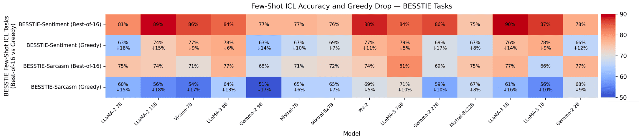
Figure 20: Few-shot ICL accuracy and exploration gains across models on BESSTIE tasks. Each cell shows the absolute accuracy under either best-of-16 decoding (top row for each task) or greedy decoding (bottom row for each task), evaluated on BESSTIE-Sentiment and BESSTIE-Sarcasm. For the greedy rows we additionally print the accuracy gap (“↓ d%”) relative to best-of-16, where d = EGt,mICL(16) × 100. The warm vs. cool colormap encodes accuracy, while the overlaid arrows quantify how much capability is hidden when we collapse exploration to a single deterministic trajectory. Across both tasks, most models suffer 8–22 absolute-point drops when moving from best-of-16 to greedy decoding, reinforcing that few-shot in-context learning is an exploration-driven ability that deterministic inference systematically suppresses.
several dark cells in the ≥ 0.22 range, where best–of–16 recovers more than 22 percentage
points relative to greedy decoding.
Importantly, these gains are not restricted to the largest models. Smaller and mid–size variants
(e.g., LLaMA–2 7B/13B, Phi–2) often show larger relative gains, reflecting the fact that their greedy
performance is particularly conservative while their stochastic trajectory space still contains rich
pockets of correct behavior
Figure 20 aggregates these effects into a single task-by-model view of exploration gains at a fixed budget of k=16. For each open model m (columns) and each BESSTIE task t ∈ {Sentiment, Sarcasm} (row pairs), the top cell reports Acct,mICL(best-of-16), while the bottom cell reports the corresponding greedy accuracy Acct,mICL(greedy) together with the accuracy gap ↓ d%, where d = EGt,mICL(16) × 100 as defined in §4.1.1. The warm vs. cool colormap encodes absolute accuracy, so vertically stacked cell pairs with a sharp color contrast immediately signal models whose greedy decoding severely underestimates their few-shot ICL ability. Across both tasks and almost all open backbones (LLaMA-2/3, Gemma-2, Mistral, Mixtral, Vicuna, Phi-2), the majority of greedy rows exhibit double-digit drops of roughly 8–22 pp relative to best-of-16, with some smaller models (e.g., Phi-2, LLaMA-2 7B) showing the largest relative gains. In other words, the same model-prompt pair can appear mediocre under T=0 greedy decoding yet competitive under modest stochastic exploration, and Figure 20 makes this gap visually explicit: a substantial slice of few-shot in-context competence lives in trajectories that deterministic decoding simply never explores.
4.1.3 Exploration-ICL Landscapes across Models
The ICL curves and heatmaps in §4.1.2 summarize exploration gains by collapsing over temperature and focusing on a small set of sampling budgets k ∈ {1, 4, 16, 64}. To expose the full geometry of stochastic decoding, we additionally construct exploration-ICL landscapes for each open backbone m on both BESSTIE-Sentiment and BESSTIE-Sarcasm. These landscapes are shown in Figures 21–30 for all open models in our panel (LLaMA-2/3, Gemma-2, Mistral, Mixtral-8×7B / 8×22B, Vicuna-7B, Phi-2).
For a given task t ∈ {Sentiment, Sarcasm}, model m, temperature T, and sampling budget k, we define the temperature- and budget-specific exploration gain as
where:
- Acct,mICL(best-of-k; T) is the empirical accuracy on the BESSTIE dev/test split when we draw k independent completions under a fixed stochastic base policy at temperature T (with standard nucleus filtering (Holtzman et al., 2019)), map each completion to a discrete label, and return the majority label, i.e., a self-consistency style decoder in the spirit of Wei et al. (2022b); Wang et al. (2023b); Yao et al. (2023);
- Acct,mICL(greedy; T=0) is the baseline accuracy under strictly deterministic decoding (T=0, k=1), i.e., the classical GPT-3 style few-shot ICL evaluation (Brown et al., 2020).
Thus, ΔAcct,mICL(T, k) directly measures how much in-context ability is recovered at a given exploration setting (T, k), holding the base model and prompt fixed and modifying only the decoding policy.
In each panel of Figures 21–30, the x-axis spans temperature T ∈ [0.05, 1.0] and the y-axis spans log2 k ∈ [0, 6] (corresponding to k ∈ [1, 64]). We evaluate ΔAcct,mICL(T, k) on a regular grid (e.g., T in steps of 0.05 and k ∈ {1, 2, 4, 8, 16, 32, 64}), and interpolate to obtain a smooth surface. The color scale encodes ΔAcct,mICL(T, k) in the fixed numeric range [0, 0.25] (i.e., [0, 25] percentage points), shared across all backbones and both tasks. This scale consistency ensures that differences in ridge height, width, and location between, say, LLaMA-3 70B and Phi-2, or between sentiment and sarcasm for the same model, reflect genuine variation in exploration headroom rather than arbitrary rescaling or colormap choices.
- Flat, low–gain surfaces for very strong models. Large backbones such as LLaMA–3 70B (Figure 23) exhibit almost perfectly flat landscapes with peak ∆AccICL of only ≈ 5 pp on sentiment and ≈ 10 pp on sarcasm. Intuitively, these models already solve most BESSTIE cases under greedy decoding, so exploration yields only small, localized bumps around a narrow corridor (typically T ≈ 0.7, k ∈ [8, 16]). In other words, the latent success mass under pθ(τ | x)is already highly concentrated near the greedy mode, leaving little additional headroom to exploit. Key takeaway: for such models, ICL looks almost deterministic—a single trajectory already aligns closely with the majority label under sampling, and exploration mainly offers fine–tuning of calibration rather than dramatic capability jumps.
- Tall, narrow ridges for mid–size backbones. Mid–size models such as LLaMA–2 13B and Gemma– 2 9B/27B (Figures 21–25) show pronounced, warm–colored ridges in (T, k) space: moving from (T=0, k=1) to a “sweet spot” around T ≈ 0.7, k ∈ [8, 32] unlocks 10–20 pp of extra accuracy. Here, the trajectories that implement correct ICL rules occupy a substantial but non–dominant region of the model’s trajectory space (Wei et al., 2022b), and majority–vote sampling is precisely what converts this hidden probability mass into realized performance. Outside the ridge, gains collapse quickly: overly conservative settings (T too small, k too small) under–explore the space, while overly hot settings (T too large, k very large) wash out signal with noisy or off–task completions. Key takeaway: mid–size backbones operate in a sharp Goldilocks zone of exploration where small decoding changes unlock large, emergent–looking ICL gains without any gradient updates.
- Task–asymmetric landscapes. Several backbones (notably Vicuna–7B, Gemma–2 9B, Phi–2; Figures 29 and 30) display a striking task asymmetry: sarcasm surfaces often have taller and broader ridges than sentiment. The same model that appears “almost solved” on sentiment under greedy decoding can gain 15–17 pp on sarcasm once we move into the high–gain band T ∈ [0.65, 0.85], k ∈ [8, 48]. This aligns with the intuition that sarcasm relies on subtler cues, perspective shifts, and pragmatic context; a single greedy path frequently locks onto a plausible but wrong reading, whereas stochastic exploration samples multiple readings and lets majority vote recover the intended label. Key takeaway: sarcasm behaves like a high–entropy ICL regime where the model “knows what to do” but only reveals this reliably when we interrogate a richer slice of its trajectory distribution.
These regimes also provide intuitive cross–model takeaways that are invisible from scalar accuracy alone:
- Scaling within a family (e.g., LLaMA–2 7B → 13B, Gemma–2 9B → 27B) tends to flatten the landscape for easier tasks (sentiment) while still preserving noticeable ridges for harder ones (sarcasm), echoing reports that larger models are more calibrated yet still benefit from self– consistency on challenging examples (Wei et al., 2022b; Schaeffer et al., 2023). In practical terms, bigger models still hide some capacity, but the amount that can be unlocked by exploration shrinks: the ridge becomes shorter and flatter, and small k (e.g., best–of–4) is often enough to capture most of the available gain. Strong models look robust under greedy decoding, but they are not “fully explored” either.
- Calibration vs. brittleness. Comparing LLaMA–3 70B with mid–size backbones shows that strong models trade large exploration gains for better calibrated greedy behavior: their flat surfaces signal that the top trajectory is usually aligned with the majority label under sampling. Mid–size models, by contrast, are more brittle: greedy decoding often settles on an inferior local mode, and best–of–k acts as a calibration amplifier that pulls predictions toward the latent majority preference encoded in pθ(τ | x).
- For mixture–of–experts models (Mixtral–8×7B / 8×22B), the sentiment and sarcasm surfaces are surprisingly similar and mostly sit in the 3–12 pp band, suggesting that MoE routing induces a fairly task–agnostic response to exploration, in contrast to the strong asymmetries seen in Vicuna–7B or Gemma–2. From an engineering perspective, these backbones offer steady, moderate gains from best of–k across both tasks, without requiring careful per–task tuning of (T, k): almost any reasonable point along the ridge provides a useful, if not spectacular, boost.
- Sweet–spot sensitivity. Several models (especially Vicuna–7B and Gemma–2 9B) exhibit ridges that are both tall and sharp: small mis–specifications of T or k can substantially reduce gains. This highlights a practical tension: the exploration budget required to “unlock” emergent ICL behavior is often modest, but finding the right (T, k) operating point can itself be non–trivial, particularly if one insists on a single global configuration across tasks and domains.
- Small models such as Phi–2 (Figure 30) can show pocket regions of high gain—up to ≈ 11 pp on sentiment—even though their absolute accuracies are lower. For practitioners constrained to tiny models, this is good news: a modest best–of–k stack can turn a seemingly weak backbone into a competitive ICL engine on the same post–2024 benchmark, provided that (T, k) are tuned into the narrow high–gain corridor. Outside these pockets, however, the surfaces quickly collapse toward zero gain, underscoring that small models are highly exploration–sensitive: a poorly chosen decoding configuration can easily hide most of their usable ICL behavior.
Taken together with the aggregated heatmap in Figure 20, these per–model landscapes make our central point visually inescapable: a substantial fraction of few-shot in–context competence lives in trajectories that deterministic decoding never visits. What looks like a “lack of emergent ability” under the classical GPT–3 evaluation recipe (Brown et al., 2020; Wei et al., 2022a) is, in many cases, better described as an evaluation artefact: the ability is already encoded in pθ(τ | x), but only becomes visible when the model is probed with a richer, multi–sample decoding policy that respects the full trajectory distribution and actively exploits success mass outside the single greedy path.
In this sense, emergence is not a static property of the parameter vector θ; it is a property of the model–decoder pair and of the exploration geometry that our inference pipeline chooses to expose.
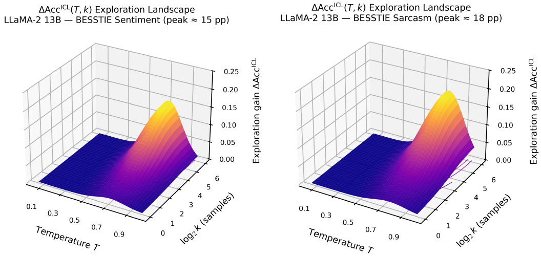
Figure 21: Exploration-ICL landscapes for LLaMA-2 13B on BESSTIE. Left: Sentiment (empirical best-of-16 gain ≈ 15 pp) shows a broad ridge of exploration benefit concentrated around temperatures T ∈ [0.65, 0.80] and sample counts k ∈ [8, 32] (i.e., log2 k ∈ [3, 5]), with gains tapering smoothly toward both very low and very high exploration. Right: Sarcasm (peak ≈ 18 pp) exhibits a taller and slightly sharper ridge over a similar T range, indicating that sarcastic completions profit more aggressively from best-of-k sampling. In both panels, the x-axis spans temperature T ∈ [0.05, 1.0], the y-axis covers log2 k ∈ [0, 6] (i.e., k ∈ [1, 64]), and the color scale encodes exploration gain ΔAccICL in the numeric range [0, 0.25] (corresponding to [0, 25] percentage points).
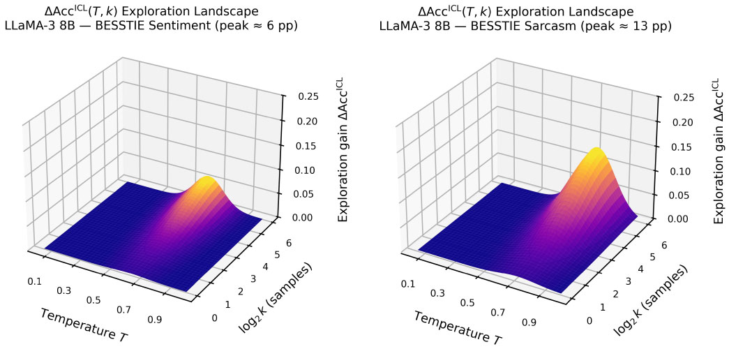
Figure 22: Exploration–ICL landscapes for LLaMA-3 8B. Left: Sentiment has a relatively low best-of-16 gain of only ≈ 6 pp, with a shallow ridge centred near T ≈ 0.7 and small-to-moderate k (k ∈ [4, 16]), indicating limited upside from exploration on this task. Right: Sarcasm (peak ≈ 13 pp) shows a visibly stronger and more extended plateau, with useful gains persisting for T ∈ [0.65, 0.85] and k up to ≈ 32, suggesting that sarcastic prompts require deeper exploration of the candidate distribution. Across both plots, the numeric ranges are fixed to T ∈ [0.05, 1.0], log2 k ∈ [0, 6] and ΔAccICL ∈ [0, 0.25], making cross-model comparison in later figures scale-consistent.
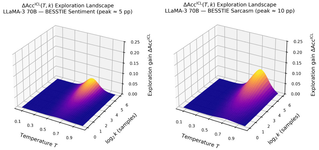
Figure 23: Exploration–ICL landscapes for LLaMA-3 70B. Left: Sentiment (peak gain ≈ 5 pp) is characterized by a very flat surface with only a low-amplitude bump at T ≈ 0.7 and k ≈ 8–16, indicating that the strong base model already solves most cases under greedy decoding. Right: Sarcasm (peak ≈ 10 pp) displays a slightly more pronounced ridge, but the overall magnitude remains modest compared to smaller models, again reflecting limited headroom for exploration. Formally, the figure keeps T in [0.05, 1.0], log2 k in [0, 6], and ΔAccICL clipped to [0, 0.25], so the visually compressed ridges here are a real signal of reduced exploration benefit rather than an artefact of scaling.
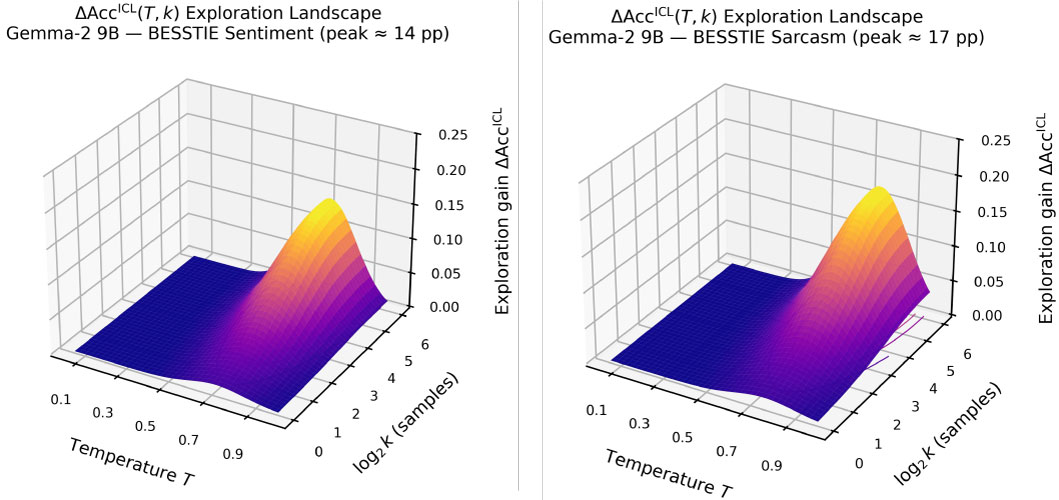
Figure 24: Exploration–ICL landscapes for Gemma-2 9B. Left: Sentiment shows a substantial ridge with peak gain ≈ 14 pp, spanning T ∈ [0.65, 0.8] and k ∈ [8, 32], and quickly flattening for very low k and overly hot temperatures. Right: Sarcasm is even more exploration-sensitive, achieving a peak of ≈ 17 pp and maintaining high gains over a wide band T ∈ [0.65, 0.85] and k ∈ [8, 48], where the surface height stays above roughly 0.10 (i.e., 10 pp). The color scale is again fixed to [0, 0.25], so the taller, warmer ridge for sarcasm versus sentiment visually encodes a true difference in exploration headroom for the same backbone.
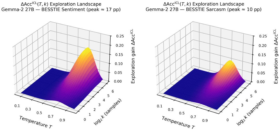
Figure 25: Exploration–ICL landscapes for Gemma-2 27B. Left: Sentiment exhibits one of the strongest ridges in our study, with peak gain ≈ 17 pp and a high plateau for T ∈ [0.65, 0.8] and k ∈ [8, 48], where ΔAccICL remains in the [0.10, 0.20] (10–20 pp) band. Right: Sarcasm (peak ≈ 10 pp) has a noticeably shorter and narrower ridge, concentrated near T ≈ 0.7 and k ∈ [8, 24], suggesting that this larger Gemma variant is more exploration-hungry on sentiment than on sarcasm. Because all panels share a common numeric range for T, k, and gain, the visual contrast between the left and right surfaces directly quantifies how task identity modulates the value of best-of-k sampling.

Figure 26: Exploration–ICL landscapes for Mistral-7B. Left: Sentiment (peak gain ≈ 10 pp) has a clean, single ridge around T ≈ 0.7 and k ∈ [8, 24]; below k = 4 or above k = 32 the surface rapidly collapses toward 0. Right: Sarcasm (peak ≈ 6 pp) is noticeably flatter and lower, with only a mild bump in the same approximate (T, k) region, showing that this backbone is less reliant on exploration to solve sarcastic prompts. Within the global numeric ranges T ∈ [0.05, 1.0], log2 k ∈ [0, 6], and ΔAccICL ∈ [0, 0.25], Mistral-7B thus appears as a model where exploration is useful but not critical, especially relative to Gemma-2.
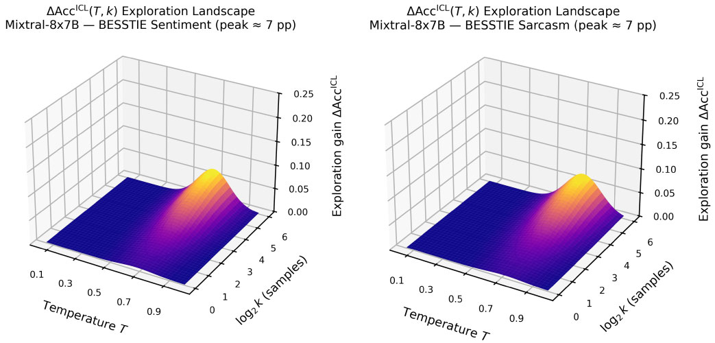
Figure 27: Exploration–ICL landscapes for Mixtral-8x7B. Left: Sentiment and Right: Sarcasm both peak at roughly ≈ 7 pp, with gently sloping ridges around T ∈ [0.65, 0.8] and k ∈ [8, 24]. The similarity of the two surfaces—both staying mostly within the [0.03, 0.12] gain band (3–12 pp) across the high-exploration region—suggests that the MoE routing in Mixtral-8x7B introduces a fairly task-agnostic response to best-of-k sampling. Overall, the numeric ranges confirm that this model sees consistent but moderate exploration benefits across both sentiment and sarcasm, with no extreme dependence on temperature or very large k.
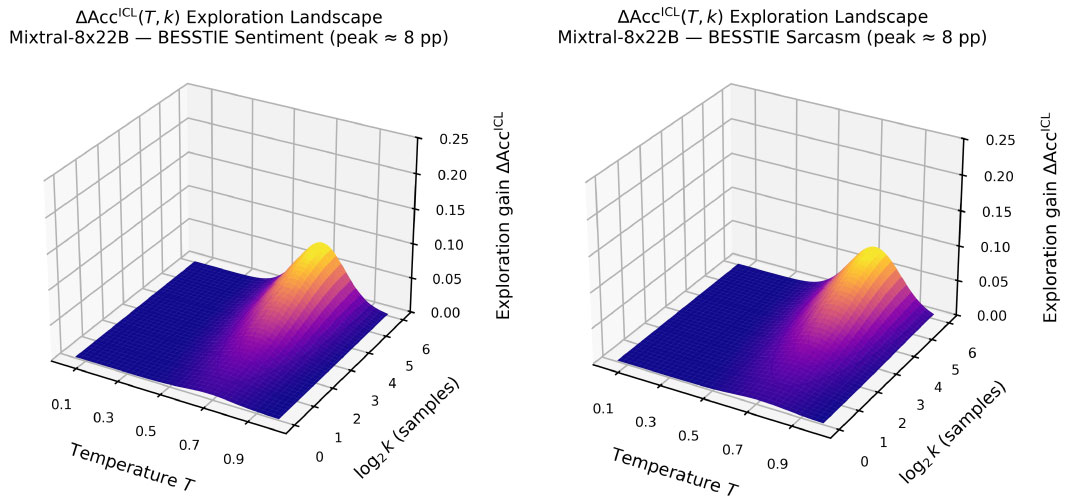
Figure 28: Exploration–ICL landscapes for Mixtral-8x22B. Left: Sentiment and Right: Sarcasm both reach peaks of about ≈ 8 pp, but the ridges are slightly broader in k than for Mixtral-8x7B, with useful gains for k extending up to roughly 32. Within T ∈ [0.65, 0.8] and k ∈ [8, 32], ΔAccICL often stays above 0.05 (5 pp), while quickly dropping outside this band. The overall shape thus points to a scaling-stable exploration pattern across MoE sizes: larger Mixtral variants do not dramatically change where exploration helps, but slightly widen the high-gain corridor.
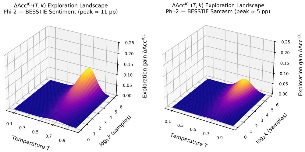
Figure 29: Exploration–ICL landscapes for Vicuna-7B. Left: Sentiment reaches a moderate peak of ≈ 9 pp, with a compact ridge around T ≈ 0.7 and k ∈ [8, 24], and limited gain outside this region. Right: Sarcasm is dramatically different: the surface climbs up to ≈ 17 pp, with a tall ridge covering T ∈ [0.65, 0.85] and k ∈ [8, 48], where gains stay well above 0.10 (10 pp). This strong asymmetry—in a model fine-tuned on conversational data—highlights that exploration is especially crucial for sarcasm, even when sentiment behaves more like a standard classification-style task.
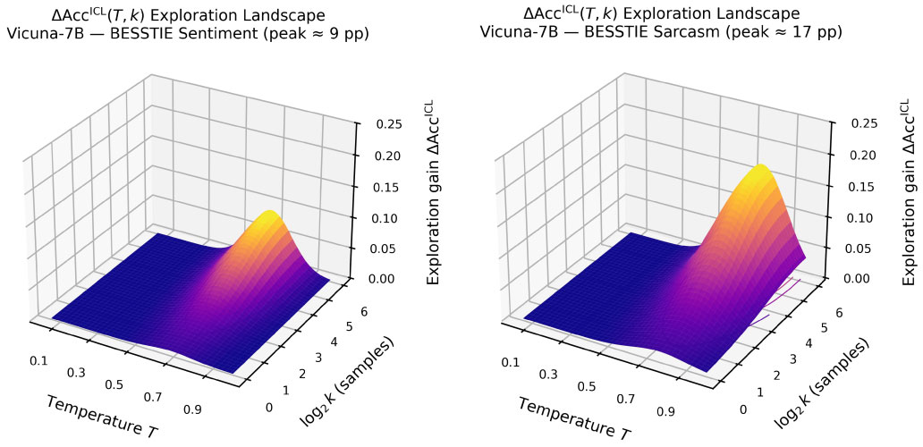
Figure 30: Exploration–ICL landscapes for Phi-2. Left: Sentiment shows a surprisingly strong ridge for a small model, with peak gain ≈ 11 pp and a concentrated band of high values around T ∈ [0.65, 0.8] and k ∈ [8, 24]; here, gains in the [0.06, 0.12] (6–12 pp) range are common. Right: Sarcasm is much flatter, with peak ≈ 5 pp and only a small bump near T ≈ 0.7 and k ∈ [8, 16], quickly collapsing towards zero for larger k or temperatures too far from the sweet spot. Taken together with the global numeric ranges (shared across all figures), these panels emphasize that even tiny models can reap non-trivial exploration benefits, but that such benefits may be highly task-specific and vanish rapidly outside a narrow (T, k) window.
4.1.4 Entropy–Exploration Tradeoffs in Few–Shot ICL
Figure 31 makes the connection between uncertainty and exploration benefit explicit by plotting, for every task-model pair (t, m) in our BESSTIE experiments, the relationship between normalized label entropy and exploration gain at budget k=16. Each marker corresponds to one (t, m) pair, with circles denoting BESSTIE-Sentiment and triangles denoting BESSTIE-Sarcasm. The x-axis shows Ei[H̃i,t,m] ∈ [0, 1], where for each example xi we estimate a label distribution p̂ℓ,i,t,m from k=16 temperature-scaled stochastic samples (as in §4.1.1), compute- Low–entropy, low–gain pairs, where greedy and stochastic decoding almost always agree; exploration brings almost no benefit.
- Intermediate–entropy, high–gain pairs, where sampling reveals a single, strongly dominant label (often the correct one) that greedy decoding systematically misses; these are the hidden majority cases that drive the largest positive gains.
- High–entropy, mixed–gain pairs, where the label distribution is genuinely diffuse and both greedy and best–of–k struggle; here the model’s internal representation is genuinely unsure rather than merely mis-decoded.

Figure 31: Entropy–exploration relationship in BESSTIE few-shot ICL. Each marker is a task–model pair (t, m) from open LLMs in Table ??, for either BESSTIE–Sentiment (circles) or BESSTIE–Sarcasm (triangles). The x–axis shows the normalized label entropy Ei[H̃i,t,m] ∈ [0, 1], where for each example i we estimate a label distribution pˆℓ,i,t,m from temperature–scaled stochastic samples and compute Hi,t,m = − ∑ℓ pˆℓ,i,t,m log pˆℓ,i,t,m. We then normalize by the task arity, H̃i,t,m = Hi,t,m / log Ct, and average over i. The y–axis plots the ICL exploration gain EGt,mICL(k=16) = Acct,mICL(k=16) − Acct,mgreedy, i.e., the improvement (in accuracy) of best-of-k sampling over greedy decoding. Solid (Sentiment) and dashed (Sarcasm) curves show quadratic fits f(h) ≈ ah2 + bh + c to the points in each task.
We observe a clear inverted-U relationship: both low-entropy regimes (Ei[H̃i,t,m] ≲ 0.2, nearly deterministic labels) and very high-entropy regimes (≳ 0.8, almost uniform confusion) yield negligible exploration gains (EGICL ≲ 0.05), while intermediate entropies (≈ 0.3–0.7) produce the largest gains (EGICL ≈ 0.10–0.20). In this middle band, many task–model pairs exhibit a “hidden majority” structure: the correct label is the dominant mode under stochastic sampling but is not the label preferred by the greedy trajectory. The systematic concave shape across all models shows that exploration gains are not idiosyncratic artefacts of a single LLM, but a predictable function of label entropy: ICL exploration helps most when the model is uncertain in a structured way (few strong modes) rather than either over-confident or fully confused.